Spark 3.0: First hands-on approach with Adaptive Query Execution (Part 3)

Spark 3.0: First hands-on approach with Adaptive Query Execution (Part 3)

In the previous articles (1)(2), we started analyzing the individual features of Adaptive Query Execution introduced on Spark 3.0. In particular, we analyzed “dynamically coalescing shuffle partitions” and “dynamically switching join strategies”. Last but not least, let’s analyze what will probably be the most-awaited and appreciated feature:

Dynamically optimizing skew joins

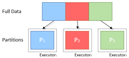
To understand exactly what it is, let’s take a moment’s step back with the theory, remembering that a DataFrame is on Spark an abstraction from the concept of RDD, which is in turn a logical abstraction of the dataset that can be processed in a distributed way thanks to the concept of partition. A dataset on Spark, once “transformed” into RDD, is divided into partitions where ideally the data is distributed in a balanced way:

In practice, it is very common for RDDs generated by certain operations (such as key grouping) to be unbalanced:

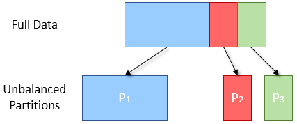
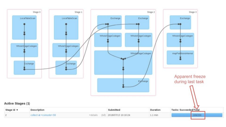
The unfortunate consequence of this is that, since computation parallels are based on the concept of data partitioning, we will not be able to adequately exploit the resources of the cluster. Identifying such situations is fairly straightforward by using the Spark UI. How many of you who are regular users of Spark will certainly have found yourself in the unpleasant situation, during which the progress bar related to an operation stops for a long time on the last tasks, giving the feeling, in the most “serious” cases, that the job has gone into freeze.

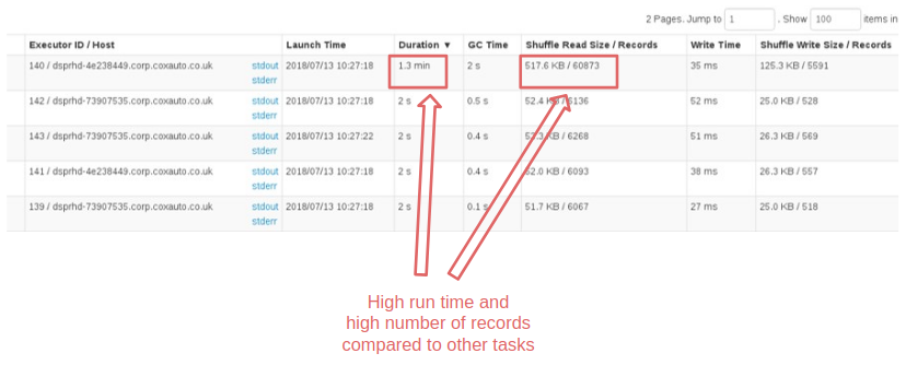
Analyzing the tasks in detail, it is easy to identify the “incriminated” ones by looking at the duration, size and number of records processed that will be one or more orders of magnitude larger than all the others.

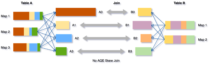
Techniques such as adding additional join keys (where possible) or key salting were used to resolve these situations without AQE. With an additional effort from developers for implementation, testing etc.

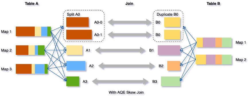
AQE mechanisms transparently discover and optimize implementation.

Let’s see how to enable the feature and set configuration parameters correctly. The core directive spark.sql.adaptive.skewJoin.enabled is set to true by default. As in the previous cases, it is sufficient to enable AQE (spark.sql.adaptive.enabled) to take advantage of the optimization in question.

To find out what policy Spark uses to identify a skewed partition, simply analyze the sources of the org.apache.spark.sql.execution.adaptive.OptimizeSkewedJoin class (class that extends Rule[SparkPlan]).

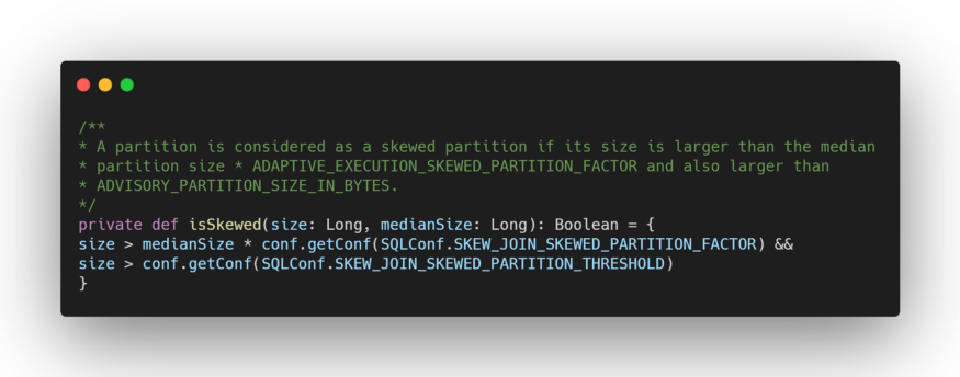
where ADAPTIVE_EXECUTION_SKEWED_PARTITION_FACTOR corresponds to the configuration property spark.sql.adaptive.skewJoin.skewedPartitionFactor and SKEW_JOIN_SKEWED_PARTITION_THRESHOLD to spark.sql.adaptive.skewJoin.skewedPartitionThresholdInBytes which ideally needs to be larger than the property spark.sql.adaptive.advisoryPartitionSizeInBytes we’ve already seen about the shuffle partitions coalesce. By default, the threshold is set to 256Mb.

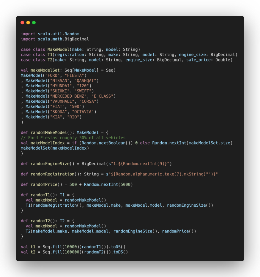
To show how this optimization works, we’ll borrow the excellent example of the article “The Taming of the Skew” based on two hypothetical tables in a car manufacturer’s database:

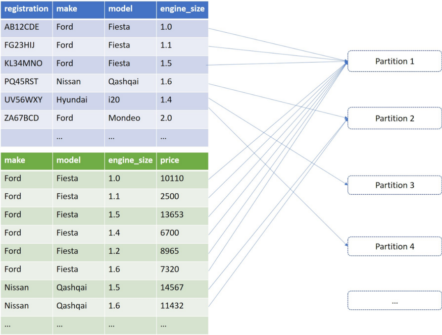
That will be created ad-hoc with an imbalance in the number of records related to one of the join keys (represented by the brand (make) and model pair).

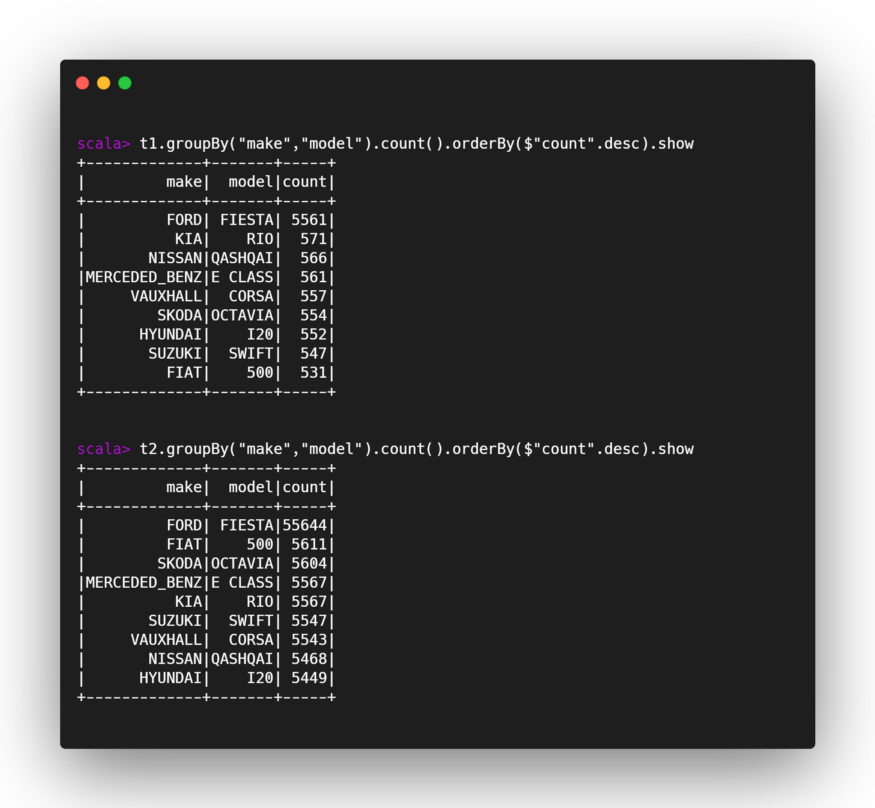
Let’s check that the keys are really unbalanced:

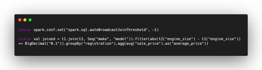
Now let’s try to join with AQE disabled (we also disable broadcast joins as the tables are very small and would frustrate the result of our experiment):

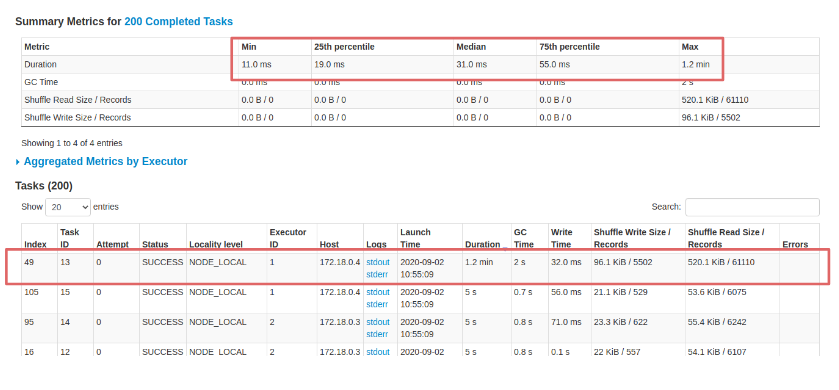
and let’s analyze the results. The longest task took, as we would have expected, a good 1.2 minutes out of 1.3 minutes total having processed most of the data concentrated on a single partition.

Now let’s repeat the experiment with AQE enabled and the configuration properties set appropriately based on the size of the sample data we’re using:

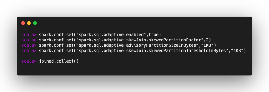
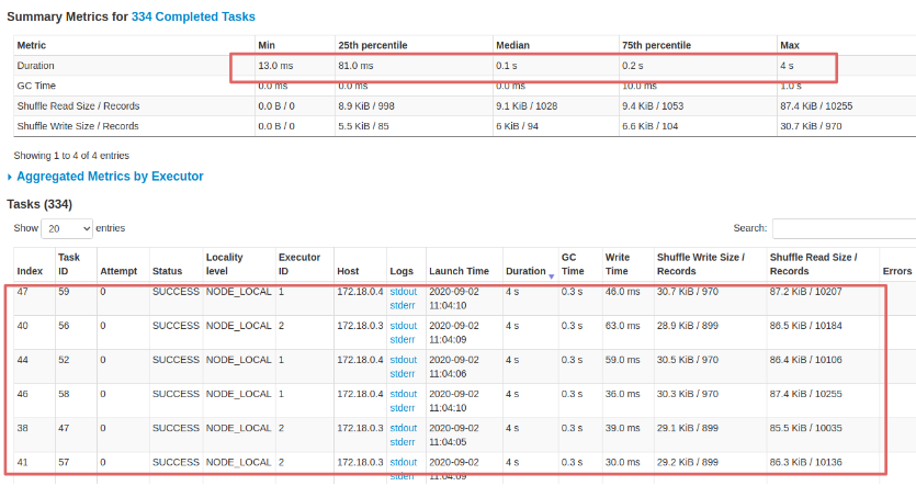
First of all, we note that the execution time drops from 1.3 min to 34 seconds. And that longer tasks now only take 4 seconds. Working fine-tuning on the parameters, I am convinced that we could get even better performance but for what was our purposes we stop here.

If you want to read the previous parts of the article:

Part 1- Dynamically coalescing shuffle partitions

Part 2 - Dynamically switching join strategies

 If you found this article useful, take a look at our Knowledge Base and follow us on Agile Lab Engineering, our Medium Publication.