Spark 3.0: First hands-on approach with Adaptive Query Execution (Part 1)

Apache Spark is a distributed data processing framework that is suitable for any Big Data context thanks to its features. Despite being a relatively recent product (the first open-source BSD license was released in 2010, it was donated to the Apache Foundation) on June 18th the third major revision was released that introduces several new features including adaptive Query Execution (AQE) that we are about to talk about in this article.

A bit of history

Spark was born, before being donated to the community, in 2009 within the academic context of ampLab (curiosity: AMP is the acronym for Algorithms Machine People) of the University of California, Berkeley. The winning idea behind the product is the concept of RDD, described in the paper “Resilient Distributed Datasets: A Fault-Tolerant Abstraction for In-Memory Cluster Computing” whose lead author is Spark Matei Zaharia’s “father”.

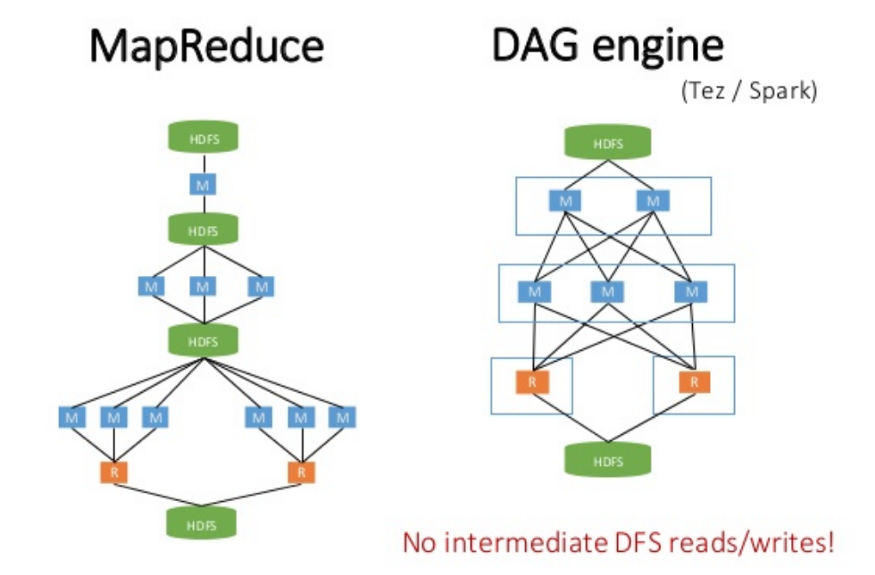
The idea is for a solution that solves the main problem of the distributed processing models available at the time (MapReduce in the first place): the lack of an abstraction layer for the memory usage of the distributed system. Some complex algorithms that are widely used in big data, such as many for training machine learning models, or manipulating graph data structures, reuse intermediate processing results multiple times during computation. The “single-stage” architecture of algorithms such as MapReduce is greatly penalized in such circumstances since it is necessary to write (and then re-read) the intermediate results of computation on persistent storage. I/O operations on persistent storage are notoriously onerous on any type of system, even more so on one deployed due to the additional overhead introduced by network communications. The concept of RDD implemented on Spark brilliantly solves this problem by using memory during intermediate computation steps on a “multi-stage” DAG engine.

The other milestone (I leap because I enter into the merits of RDD programming and Spark’s detailed history, although very interesting, outside the objectives of the article) is the introduction on the first stable version of Spark (which had been donated to the Apache community) of the Spark SQL module.

One of the reasons for the success of the Hadoop framework before Spark’s birth was the proliferation of products that added functionality to the core modules. Among the most used surely we have to mention Hive, SQL abstraction layer over Hadoop. Despite MapReduce’s limitations that make it underperforming to run more complex SQL queries on this engine after “translation” by Hive, the same is still widespread today mainly because of its ease of use.

The best way to retrace the history of the SQL layer on Spark is again to start with the reference papers. Shark (spark SQL’s ancestor) dating back to 2013 and the one titled “Spark SQL: Relational Data Processing in Spark” where Catalyst, the optimizer that represents the heart of today’s architecture, is introduced.

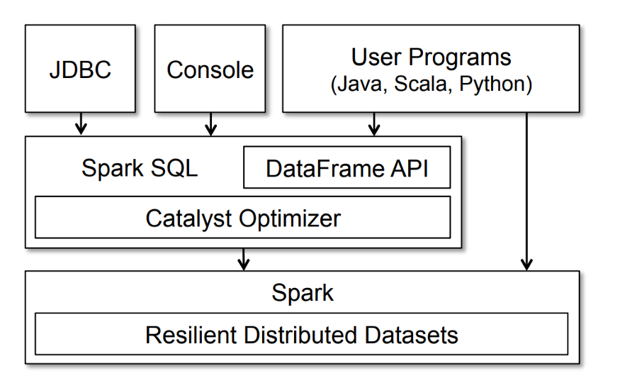
Spark SQL features are made available to developers through objects called DataFrame (or Java/Scale Datasets in type-safe) that represent RDDs at a higher level of abstraction. You can use the DataFrame API through a specific DSL or through SQL.

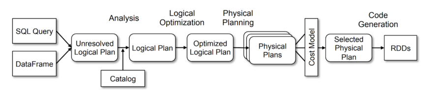
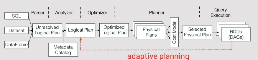
Regardless of which method you choose to use, DataFrame operations will be processed, translated, and optimized by Catalyst (Spark from v2.0 onwards) according to the following workflow:

What’s new

We finally get to get into the merits of Adaptive Query Execution, a feature that at the architectural level is implemented at this level. More precisely, this is an optimization that dynamically intervenes between the logical plan and the physical plan by taking advantage of the runtime statistics captured during the execution of the various stages according to the stream shown in the following image:

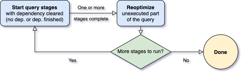
The Spark SQL execution stream in version 3.0 then becomes:

Optimizations in detail

Because the AQE framework is based on an extensible architecture based on a set of logical and physical plan optimization rules, it can easily be assumed that developers plan to implement additional functionality over time. At present, the following optimizations have been implemented in version 3.0:

• Dynamically coalescing shuffle partitions
• Dynamically switching join strategies
• Dynamically optimizing skew joins

let’s go and see them one by one by touching them with our hands through code examples.

Regarding the creation of the test cluster, we recommend that you refer to the previously published article: “How to create an Apache Spark 3.0 development cluster on a single machine using Docker”.

Dynamically coalescing shuffle partitions

Shuffle operations are notoriously the most expensive on Spark (as well as any other distributed processing framework) due to the transfer time required to move data between cluster nodes across the network. Unfortunately, however, in most cases they are unavoidable.

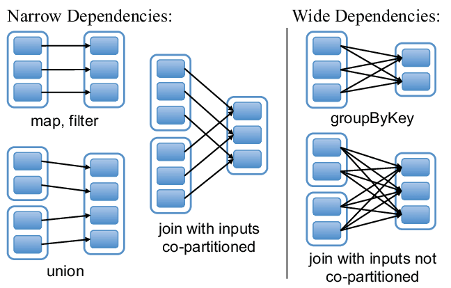
Transformations on a dataset deployed on Spark, regardless of whether you use RDD or DataFrame API, can be of two types: narrow or wide. Wide-type data needs partition data to be redistributed differently between executors to be completed. The infamous shuffle operation (and creating a new execution stage).

Without AQE, determining the optimal number of DataFrame partitions resulting from performing a wide transformation (e.g. joins or aggregations) was assigned to the developer by setting the spark.sql.shuffle.partitions configuration property (default value: 200). However, without going into the merits of the data it is very difficult to establish an optimal value, with the risk of generating partitions that are too large or too small and resulting in performance problems.

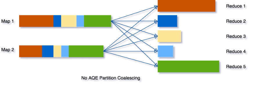
Let’s say you want to run an aggregation query on data whose groups are unbalanced. Without the intervention of AQE, the number of partitions resulting will be the one we have expressed (e.g. 5) and the final result could be something similar to what is shown in the image:

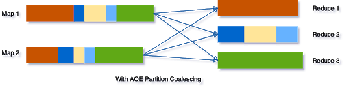
Enabling AQE instead would put data from smaller partitions together in a larger partition of comparable size to the others. With a result similar to the one shown in the figure.

This optimization is triggered when the two configuration properties spark.sql.adaptive.enabled and spark.sql.adaptive.coalescePartitions.enabled are both set to true. Since the second is set true by default, practically to take advantage of this feature you only need to enable the global property for AQE activation.

Actually going to parse the source code you find that AQE is actually enabled only if the query needs shuffle operations or is composed of sub-queries:

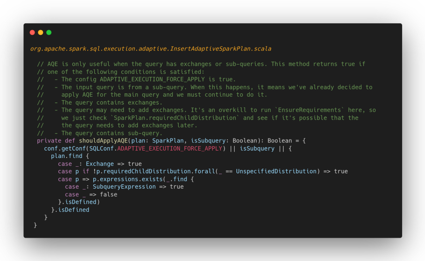
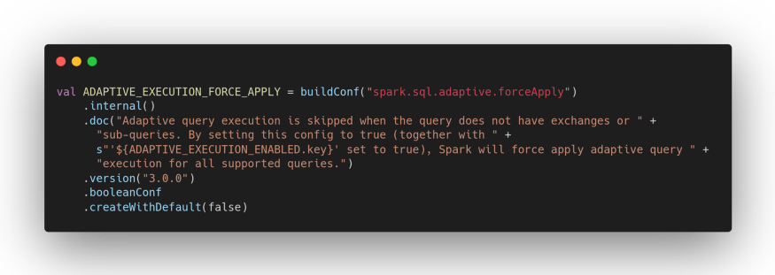
and that there is a configuration property that you can use to force AQE even in the absence of one of the two conditions above.

The number of partitions after optimization will depend instead on the setting of the following configuration options:

• spark.sql.adaptive.coalescePartitions.initialPartitionNum
• spark.sql.adaptive.coalescePartitions.minPartitionNum
• spark.sql.adaptive.advisoryPartitionSizeInBytes

where the first represents the starting number of partitions (default: spark.sql.shuffle.partitions), the second represents the minimum number of partitions after optimization (default: spark.default.parallelism), and the third represents the “suggested” size of the partitions after optimization (default: 64 Mb).

To test the behaviour of the dynamic coalition feature of AQE’s shuffle partitions, we’re going to create two simple datasets (one is to be understood as a lookup table that we need to have a second dataset to join).

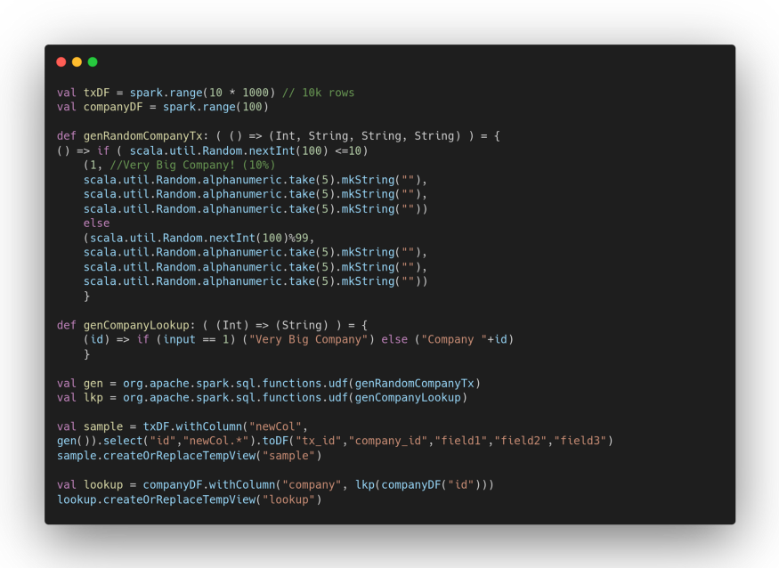
The sample dataset is deliberately unbalanced, the transactions of our hypothetical “Very Big Company” are about 10% of the total. Those of the remaining companies about 1%:

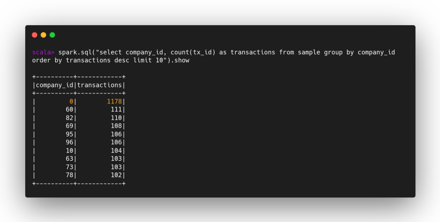
Let’s first test what would happen without AQE.

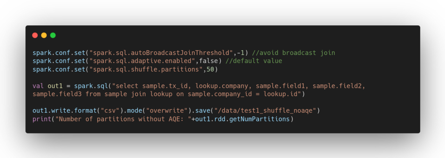
We will receive output:

Number of partitions without AQE: 50

The value is exactly what we have indicated ourselves by setting the configuration property spark.sql.shuffle.partitions.

We repeat the experiment by enabling AQE.

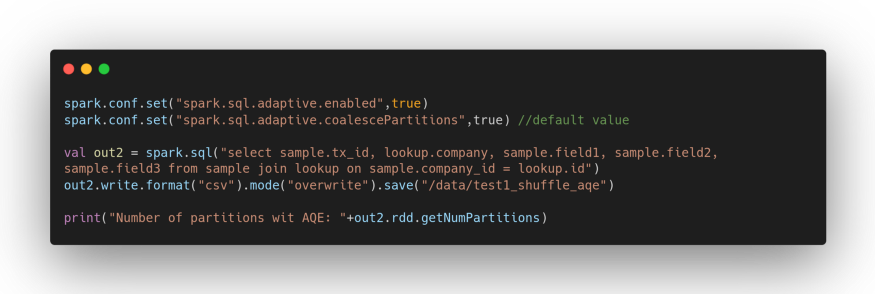
The new output will be:

Number of partitions with AQE: 7

The value, in this case, was determined based on the default level of parallelism (number of allocated cores), that is, by the value of the spark.sql.adaptive.coalescePartitions.minPartitionNum configuration property.

Now let’s try what happens by “suggesting” the target size of the partitions (in terms of storage). Let’s set it to 30 Kb which is a value compatible with our sample data.

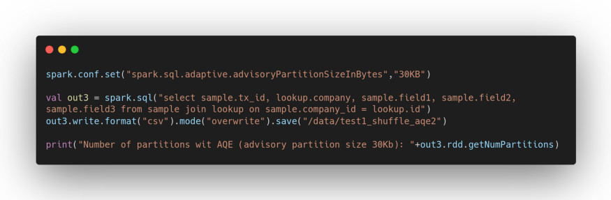
This time the output will be:

Number of partitions with AQE (advisory partition size 30Kb): 15

regardless of the number of cores allocated on the cluster for our job.

Apart from having a positive impact on performance, this feature is very useful in creating optimally sized output files (try analyzing the contents of the job output directories that I created in CSV format while being less efficient so that you can easily inspect the files).

In the second and third part of the article we will try the other two new features:

• Dynamically switching join strategies
• Dynamically optimizing skew joins.

Stay tuned!

 If you found this article useful, take a look at our Knowledge Base and follow us on our Medium Publication, Agile Lab Engineering!